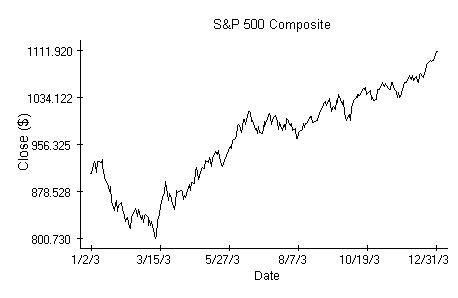
Here we would like to investigate whether it is possible from the opening values of a particular stock index, such as the Standard and Poor's 500 Composite, predict values of a particular equity. We are not looking for a specific prediction formula, but rather for evidence that such a quest is justifiable. While there is only one S&P 500 composite index, there are hundreds of equities to choose from. To find an argument that a possible dependence between the S&P 500 openings and closings of some particular stock existed for at least some period of time we consider the Dow-Jones Industrial average (DJ). The DJ average is calculated from prices of 30 stocks in a simple way. Simple enough to infer that if the closing prices of the DJ average depend on opening values of the S&P 500 then some of the DJ component closings do depend on the S&P 500 openings as well.

Technically we could proceed the same way as when we investigated the possibility of market index prediction. The associated regression analysis is in fact inevitable and does indicate that there is a relation between the DJ closings and a sequence of preceding S&P 500 openings and closings, at least with regard to data from 2003. The outcome of the analysis, which is otherwise boring, can be justified as follows. It is a common knowledge that movements of the DJ average follow closely those of S&P 500.

If the correlation between the two indices is close to one, then we can replace the regression equation in the previous note by the relation

	rcDJ[n]=b[0]+b[1]roS&P[n]+b[2]rcS&P[n-1]+e[n],
         	

where rcDJ is the return on the DJ average and roS&P, rcS&P are the respective returns on the S&P 500 index calculated from the opening and closing values. The regression analysis shows that the last equation is valid indeed, at least for the 2003 data, and the coefficients b[1] and b[2] are significant. The diagnostic plots are very similar to those in the market index prediction note.

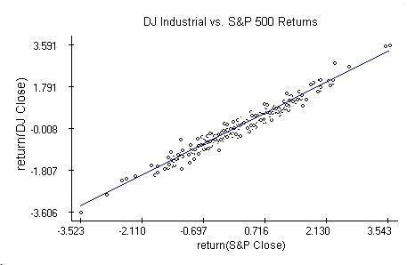
To support the naive inference leading to the above equation, the relation between DJ and S&P 500 over 2003 was investigated more thoroughly. As the diagnostic plots below indicate,

	rcDJ[n]=b S&P[n]+e[n],
		

where e[n] are independent Normal random variables and b is likely a quantity smaller than one. The coefficient is smaller than one because the 95% confidence region for b does not cover one. This also means that fund managers trying to resemble the S&P 500 had in 2003 somewhat better returns than those resembling the DJ industrial.

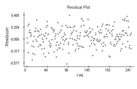
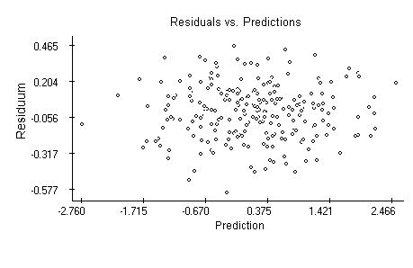
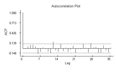
The residual plot, obtained by fitting the preceding equation, is interesting, because the variability of the residuals is more steady than what we see in simple return plots.

The autocorrelation plot indicates independence of the residuals.

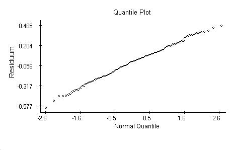
The quantile plot supports the hypothesis about normality of the residuals.

Notes

A thorough introduction to linear regression analysis is

Draper, N. and Smith, H.: Applied Regression Analysis, Second Ed., Wiley, New York, 1981.

The data used in the example are available from Yahoo finance.

Keywords

Linear regression, t-test, F-test, Cook's distance, Normal distribution, quantile plot, time series, residuals.