 View as PDF
 Introduction
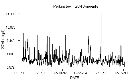
This example illustrates one possible solution to the problem how to decide if the measurements indicate a long term change in air sulfate amounts and how to quantify it. It is based on ten years of Teflon filter data describing particulate SO4 concentrations (mg/l) observed weekly since 1989 till 1998 at Perkinstown, Wisconsin, USA; see the figure. The station at Perkinstown belongs to the CASTNet air quality monitoring network operated by the US Environmental Protection Agency.
Theory
The theory for inference utilizes positiveness of the observed chemical concentration c. If c is a positive random variable then c = exp(r), where exp denotes the exponential function, and r is also a random variable. The percentage change in concentration from week n to week n+P is computed according to the formula pc[n]=100*(c[n+P] - c[n])/c[n], where c[n] is the observed concentration on week n of the sampling period and r[n] is the corresponding random variable. Using the mentioned exponential representation we get pc[n]=100*(exp(r[n+P]-r[n])-1). Notice that the percentage change pc[n] over the period P is zero if the difference r[n+P]-r[n] is zero. Consequently, the overall percentage change can be defined using the relation pc=100*(exp(m)-1), where m is the mean of differences r[n+P]-r[n]. The percentage change is considered significant if the mean deviates significantly from zero. If the average is positive then we have evidence of increase in air pollution while a significant negative average means an evidence of a decline.
Model
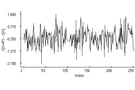
The reason for inference about r rather than about c is that, as the data indicate, r is a Gaussian stochastic process described by a periodic trend p[n], perhaps plus a linear component a+b*n, where a, b are constant numbers. More specifically, it seems that r[n]=a+b*n+p[n]+s[n], where p[n] is a periodic function with period P and s[n] is a zero-mean stochastic component. The periodicity has in consequence that r[n+P]-r[n]=b*P+e[n], where e[n]=s[n+P]-s[n], and as practice shows, e[n] is often a zero-mean stationary Gaussian stochastic process. Notice that if the periodicity and stationarity assumptions are correct then the differences r[n+P]-r[n] describing the random changes in pollutant concentrations form also a stationary Gaussian process. Due to the definition c[n]=exp(r[n]), the variable r[n]=ln(c[n]) is observable. From experience we know that the observed pollutant amounts may undergo annual seasonal changes. The trend of r is thus considered with an annual period. The Perkinstown data set is thus split in two samples from 1. 1. 1989 to 31. 12. 1993 and from 1. 1. 1994 to 31. 12. 1998. Differences of the logarithms for the Perkinstown data are in the figure above. The period P is 5 years; recall that a function with an annual periodicity has also a five-year period. The familiar Box-Jenkins exploratory time-series analysis is based on the quantile and partial autocorrelation plots.
Inference
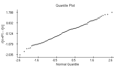
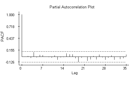
The quantile plot indicates that the differences may be generated by Normal random variables with the same mean and variance. The autocorrelation plot indicates the differences are independent. The attempt to model the series using a first-order autoregression shows that the autoregressive coefficient in the model is not significantly different from zero. The differences r[n+P]-r[n] may thus well be generated by a sequence of independent, identically distributed Normal random variables and we can use a one-sample t-test to decide if their average differs significantly from null. The t-test outcome favors a significant percentage decline in concentrations over the five-year period.
Data
The data used in the example are (in different units) available at the EPA CASTNet web site http://www.epa.gov/castnet/data.
References
J. Mohapl: Assessment of changes in pollutant concentrations. Environmental Monitoring & Assessment , 111-200. Handbook of Environmental Monitoring, edited by Prof. Bruce Wiersma and published by CRC Press 2004
P. J. Brockwell and R. A. Davis: Time Series: Theory and Methods. Springer-Verlag, New York, Berlin, Heidelberg, Tokyo 1987