Introduction

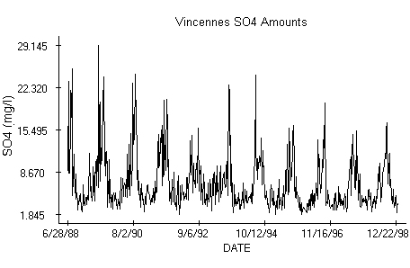
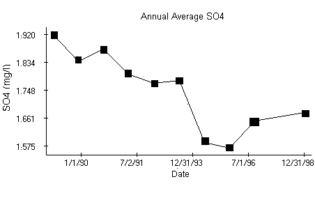
The decision if a change in a long series of data occurred is, sometimes, more important than an absolute value of the change. The ways to decide about significance of such a change are many. One possibility is to use a two-way ANOVA table, as we illustrate next on a decade of Teflon sulfate concentrations collected weekly at the Vincennes station, Indiana, USA.

Model

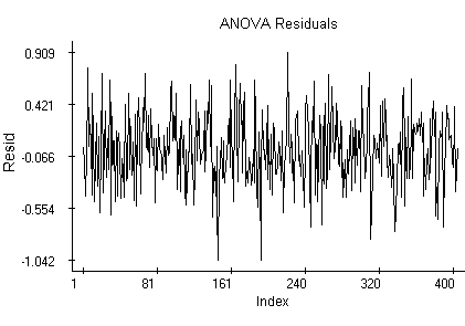
The data from the station plotted against time indicate an annual periodicity with a seemingly high variability over the summer time. The Scheffe's test applied to the data in post-hoc analysis marks a significant difference between the first year of sampling, 1989, and years 1995, 1996 when a trend reversal occurred. A logarithm transformation stabilizing variability of the Vincennes data has been applied before the sample was split in smaller, annual series that form the ANOVA table. Columns of the table, the annual series, are the treatments and the rows are the blocks. We recall that an observation in the two-way table is modeled as y[i][j] = m + a[i] + b[j] + e[i][j], where e[i][j] represent independent, identically distributed Normal random variables with zero mean. The parameters m, a[i] and b[j], i = 1, ... , 52, j = 1,..., 12, are estimated by the least-squares method with the restrictions a[1] + ... + a[52] = 0, b[1] + ... +b[12] = 0, respectively. Due to the obvious periodicity in the annual concentrations, we have no interest in testing equality of the block effects. We need them though to verify if the fundamental assumptions of ANOVA are satisfied before testing equality of the treatments. The residuals, obtained from the logarithmized observations after subtraction of the estimated trend m + a[i] + b[j], have no apparent trend.

Normality

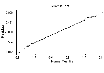
The quantile plot indicates that the same Normal distribution might generate the residuals.

Autocorrelation

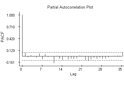
The partial autocorrelation plot admits the possibility that the data are independent. The systematically negative values in the second part of the plot could mean that the trend has not been eliminated entirely.

Testing

The Kolmogorov-Smirnov test does not reject the null hypothesis about Normal distribution of the residuals and the first two autocorrelations do not test as significant. Annual averages of the logarithms exhibit a decline till 1995, when the trend starts to increase again. The Scheffe's test points out the highest and lowest values in the plot as significant.

Limitations

The presented method has two serious limitations. It does not admit missing observations, something rather common for air quality data. The missing data must be thus estimated before the above analysis takes place. It cannot be applied to irregularly sampled data. That makes it of no use for assessment of changes in precipitation acidity, for example.

Data

The data used in the example are (in different units) available at the EPA's CASTNet web site http://www.epa.gov/castnet/data.

References

J. Mohapl: Assessment of changes in pollutant concentrations. Environmental Monitoring & Assessment , 111-200, Handbook of Environmental Monitoring, edited by Prof. Bruce Wiersma and published by CRC Press 2004

J. Mohapl: A statistical assessment of changes in precipitation chemistry at CAPMoN sites, Canada. Environmental Monitoring & Assessment, 1 - 35, 72, 2001